Service Patterns and Calendar Schedules

Overview

Each trip in a GTFS feed is referenced to a service_id (in trips.txt). The GTFS reference specifies that a “service_id contains an ID that uniquely identifies a set of dates when service is available for one or more routes”. A service could run on every weekday or only on Saturdays for example. Other possible services run only on holidays during a year, independent of weekdays. However, feeds are not required to indicate anything with service_ids and some feeds even use a unique service_id for each trip and day. In this vignette, we’ll look at a general way to gather information on when trips run by using “service patterns”.

Service patterns can be used to find a typical day for further analysis like routing or trip frequencies for different days.

Prepare data

We use a feed from the New York Metropolitan Transportation Authority. It is provided as a sample feed with tidytransit but you can read it directly from the MTA’s website. Note that some routes and services have been removed from the feed to reduce package size.

local_gtfs_path <- system.file("extdata", "nyc_subway.zip", package = "tidytransit")
gtfs <- read_gtfs(local_gtfs_path)
# gtfs <- read_gtfs("http://web.mta.info/developers/data/nyct/subway/google_transit.zip")

Tidytransit provides a dates_services (stored in the list .) that indicates which service_id runs on which date. This is later useful for linking dates and trips via service_id.

head(gtfs$.$dates_services)

## # A tibble: 6 × 2
##   date       service_id             
##   <date>     <chr>                  
## 1 2018-06-24 ASP18GEN-1037-Sunday-00
## 2 2018-06-24 ASP18GEN-2048-Sunday-00
## 3 2018-06-24 ASP18GEN-3041-Sunday-00
## 4 2018-06-24 ASP18GEN-4049-Sunday-00
## 5 2018-06-24 ASP18GEN-5048-Sunday-00
## 6 2018-06-24 ASP18GEN-6030-Sunday-00

To understand service patterns better we need information on weekdays and holidays. With a calendar table we know the weekday and possible holidays for each date. We’ll use a minimal example with two holidays.

holidays = tribble(~date, ~holiday,
  ymd("2018-07-04"), "Independence Day",
  ymd("2018-09-03"), "Labor Day")

calendar = tibble(date = unique(gtfs$.$dates_services$date)) %>% 
  mutate(
    weekday = (function(date) {
      c("Sunday", "Monday", "Tuesday", 
        "Wednesday", "Thursday", "Friday", 
        "Saturday")[as.POSIXlt(date)$wday + 1]
    })(date)
  )

calendar <- calendar %>% left_join(holidays, by = "date")
head(calendar)

## # A tibble: 6 × 3
##   date       weekday   holiday
##   <date>     <chr>     <chr>  
## 1 2018-06-24 Sunday    NA     
## 2 2018-06-25 Monday    NA     
## 3 2018-06-26 Tuesday   NA     
## 4 2018-06-27 Wednesday NA     
## 5 2018-06-28 Thursday  NA     
## 6 2018-06-29 Friday    NA

To analyse on which dates trips run and to group similar services we use service patterns. Such a pattern simply lists all dates a trip runs on. For example, a trip with a pattern like 2019-03-07, 2019-03-14, 2019-03-21, 2019-03-28 runs every Thursday in March 2019. To handle these patterns, we create a servicepattern_id using a hash function. Ideally there are the same number of servicepattern_ids and service_ids. However, in real life feeds this is rarely the case. In addition, the usability of service patterns depends largely on the feed and its complexity.

gtfs <- set_servicepattern(gtfs)

Our gtfs feed now contains the data frame servicepatterns which links each servicepattern_id to an existing service_id (and by extension trip_id).

head(gtfs$.$servicepatterns)

## # A tibble: 6 × 2
##   service_id                servicepattern_id
##   <chr>                     <chr>            
## 1 ASP18GEN-1037-Sunday-00   s_a4c6b26        
## 2 ASP18GEN-1038-Saturday-00 s_c578d4a        
## 3 ASP18GEN-1087-Weekday-00  s_e25d6ca        
## 4 ASP18GEN-2042-Saturday-00 s_c578d4a        
## 5 ASP18GEN-2048-Sunday-00   s_a4c6b26        
## 6 ASP18GEN-2097-Weekday-00  s_e25d6ca

In addition, gtfs$.$dates_servicepatterns has been created which connects dates and service patterns (like dates_services). We can compare the number of service patterns to the number of services.

head(gtfs$.$dates_servicepatterns)

## # A tibble: 6 × 2
##   date       servicepattern_id
##   <date>     <chr>            
## 1 2018-06-24 s_a4c6b26        
## 2 2018-06-25 s_e25d6ca        
## 3 2018-06-26 s_e25d6ca        
## 4 2018-06-27 s_e25d6ca        
## 5 2018-06-28 s_e25d6ca        
## 6 2018-06-29 s_e25d6ca

# number of service ids used
n_services <- length(unique(gtfs$trips$service_id)) # 52

# unique date patterns 
n_servicepatterns <- length(unique(gtfs$.$servicepatterns$servicepattern_id)) # 3

The example feed uses 52 service_ids but there are actually only 3 different date patterns. Other feeds might not have such low numbers, for example the Swiss GTFS feed uses around 15’600 service_ids which all identify unique date patterns.

Analyse Data

Exploration Plot

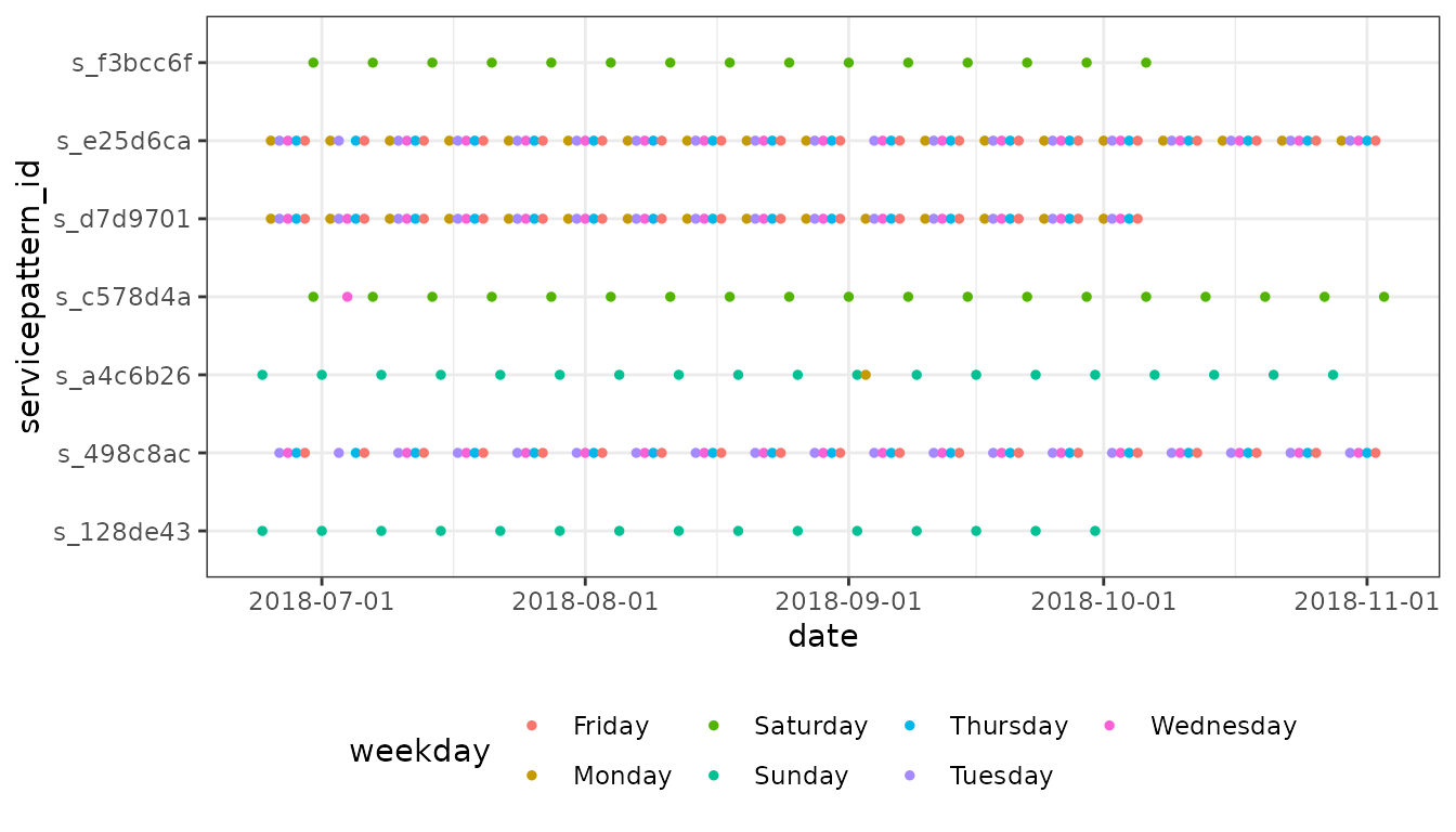
We’ll now try to figure out usable names for those patterns. A good way to start is visualising the data.

date_servicepattern_table <- gtfs$.$dates_servicepatterns %>% left_join(calendar, by = "date")

ggplot(date_servicepattern_table) + theme_bw() + 
  geom_point(aes(x = date, y = servicepattern_id, color = weekday), size = 1) + 
  scale_x_date(breaks = scales::date_breaks("1 month")) + theme(legend.position = "bottom")

The plot shows that pattern s_a4c6b26 runs on every Sunday from July until October. s_c578d4a runs every Saturday and on one Wednesday. s_e25d6ca covers weekdays (Mondays through Friday) with one exception.

Names for service patterns

It’s generally difficult to automatically generate readable names for service patterns. Below you see a semi automated approach with some heuristics. However, the workflow depends largely on the feed and its structure. You might also consider setting names completely manually.

suggest_servicepattern_name = function(dates, calendar) {
  servicepattern_calendar = tibble(date = dates) %>% left_join(calendar, by = "date")
  
  # all normal dates without holidays
  calendar_normal = servicepattern_calendar %>% filter(is.na(holiday))
  
  # create a frequency table for all calendar dates without holidays
  weekday_freq = sort(table(calendar_normal$weekday), decreasing = T)
  n_weekdays = length(weekday_freq)
  
  # all holidays that are not covered by normal weekdays anyways
  calendar_holidays <- servicepattern_calendar %>% filter(!is.na(holiday)) %>% filter(!(weekday %in% names(weekday_freq)))

  if(n_weekdays == 7) {
    pattern_name = "Every day"
  }
  # Single day service
  else if(n_weekdays == 1) {
    wd = names(weekday_freq)[1]
    # while paste0(weekday, "s") is easier, this solution can be used for other languages
    pattern_name = c("Sunday"  = "Sundays", 
        "Monday"    = "Mondays", 
        "Tuesday"   = "Tuesdays", 
        "Wednesday" = "Wednesdays",
        "Thursday"  = "Thursdays",  
        "Friday"    = "Fridays",  
        "Saturday"  = "Saturdays")[wd]
  } 
  # Weekday Service
  else if(n_weekdays == 5 && 
      length(intersect(names(weekday_freq), 
        c("Monday", "Tuesday", "Wednesday", "Thursday", "Friday"))) == 5) {
    pattern_name = "Weekdays"
  }
  # Weekend
  else if(n_weekdays == 2 && 
      length(intersect(names(weekday_freq), c("Saturday", "Sunday"))) == 2) {
    pattern_name = "Weekends"
  }
  # Multiple weekdays that appear regularly
  else if(n_weekdays >= 2 && (max(weekday_freq) - min(weekday_freq)) <= 1) {
    wd = names(weekday_freq)
    ordered_wd = wd[order(match(wd, c("Monday", "Tuesday", "Wednesday", "Thursday", "Friday", "Saturday", "Sunday")))]
    pattern_name = paste(ordered_wd, collapse = ", ")
  } 
  # default
  else {
    pattern_name = paste(weekday_freq, names(weekday_freq), sep = "x ", collapse = ", ")
  }
  
  # add holidays
  if(nrow(calendar_holidays) > 0) {
    pattern_name <- paste0(pattern_name, " and ", paste(calendar_holidays$holiday, collapse = ", "))
  }
  
  pattern_name <- paste0(pattern_name, " (", min(dates), " - ", max(dates), ")") 

  return(pattern_name)
}

We’ll apply this function to our service patterns and create a table with ids and names.

servicepattern_names = gtfs$.$dates_servicepatterns %>% 
  group_by(servicepattern_id) %>% summarise(
    servicepattern_name = suggest_servicepattern_name(date, calendar)
  )

print(servicepattern_names)

## # A tibble: 3 × 2
##   servicepattern_id servicepattern_name                                     
##   <chr>             <chr>                                                   
## 1 s_a4c6b26         Sundays and Labor Day (2018-06-24 - 2018-10-28)         
## 2 s_c578d4a         Saturdays and Independence Day (2018-06-30 - 2018-11-03)
## 3 s_e25d6ca         Weekdays (2018-06-25 - 2018-11-02)

Visualise services

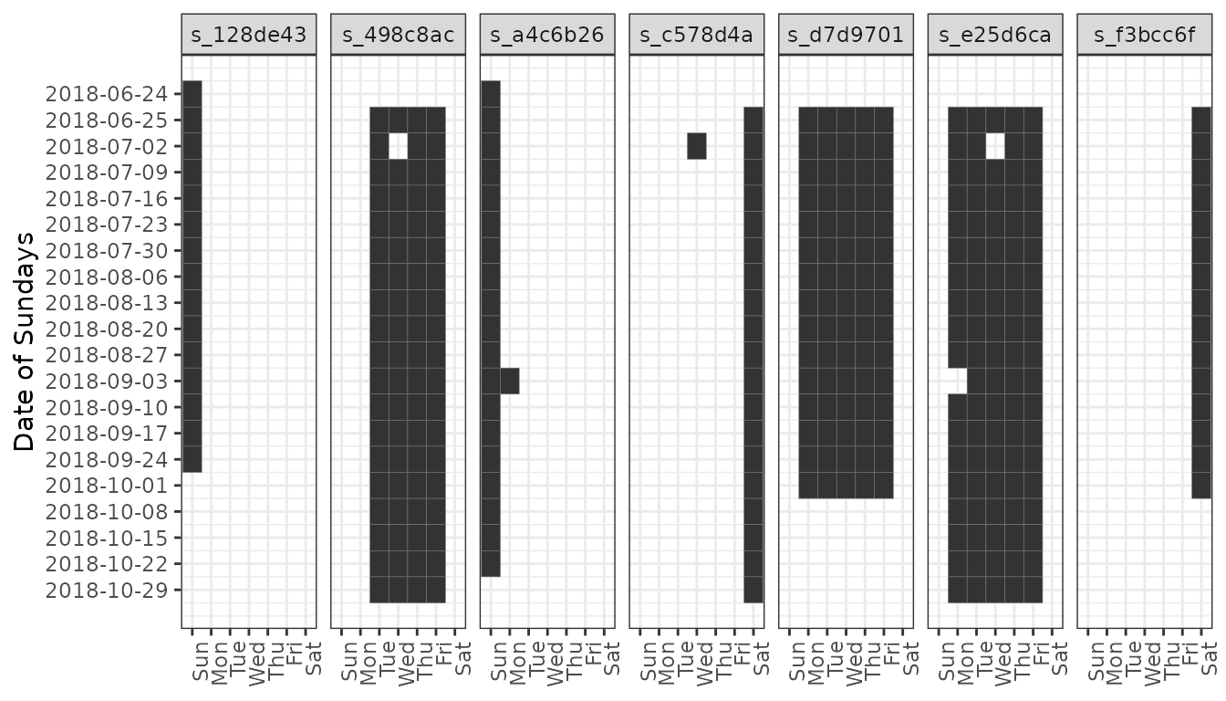
Plot calendar for each service pattern

We can plot the service pattern like a calendar to visualise the different patterns. The original services can be plotted similarly (given it’s not too many) by using dates_services and service_id.

dates = gtfs$.$dates_servicepatterns
dates$wday <- lubridate::wday(dates$date, label = T, abbr = T, week_start = 7)
dates$week_nr <- lubridate::week(dates$date)

dates <- dates %>% group_by(week_nr) %>% summarise(week_first_date = min(date)) %>% right_join(dates, by = "week_nr")

week_labels = dates %>% select(week_nr, week_first_date) %>% unique()

ggplot(dates) + theme_bw() +
  geom_tile(aes(x = wday, y = week_nr), color = "#747474") +
  scale_x_discrete(drop = F) +
  scale_y_continuous(trans = "reverse", labels = week_labels$week_first_date, breaks = week_labels$week_nr) +
  theme(legend.position = "bottom", axis.text.x = element_text(angle = 90, hjust = 1)) +
  labs(x = NULL, y = "Date of Sundays") +
  facet_wrap(~servicepattern_id, nrow = 1)

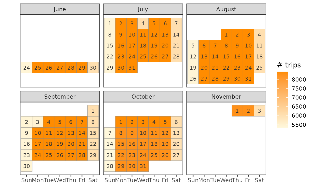
Plot number of trips per day as calendar

We can plot the number of trips for each day as a calendar heat map.

trips_servicepattern = left_join(select(gtfs$trips, trip_id, service_id), gtfs$.$servicepatterns, by = "service_id")
trip_dates = left_join(gtfs$.$dates_servicepatterns, trips_servicepattern, by = "servicepattern_id", relationship = "many-to-many")

trip_dates_count = trip_dates %>% group_by(date) %>% summarise(count = dplyr::n()) 
trip_dates_count$weekday <- lubridate::wday(trip_dates_count$date, label = T, abbr = T, week_start = 7)
trip_dates_count$day_of_month <- lubridate::day(trip_dates_count$date)
trip_dates_count$first_day_of_month <- lubridate::wday(trip_dates_count$date - trip_dates_count$day_of_month,  week_start = 7)
trip_dates_count$week_of_month <- ceiling((trip_dates_count$day_of_month - as.numeric(trip_dates_count$weekday) - trip_dates_count$first_day_of_month) / 7)
trip_dates_count$month <- lubridate::month(trip_dates_count$date, label = T, abbr = F)

ggplot(trip_dates_count, aes(x = weekday, y = -week_of_month)) + theme_bw() +
  geom_tile(aes(fill = count, colour = "grey50")) +
  geom_text(aes(label = day_of_month), size = 3, colour = "grey20") +
  facet_wrap(~month, ncol = 3) +
  scale_fill_gradient(low = "cornsilk1", high = "DarkOrange", na.value="white")+
    scale_color_manual(guide = "none", values = "grey50") +
  theme(axis.text.y = element_blank(), axis.ticks.y = element_blank()) +
  theme(panel.grid = element_blank()) +
  labs(x = NULL, y = NULL, fill = "# trips") +
  coord_fixed()

Flavio Poletti

2023-06-23