Generate a Departure Timetable

In this vignette a departure timetable for a stop is generated and visualised. For some analysis it is important to know how and when a single stop is served and workflows to gather and plot such data can help with this analysis.

Read GTFS data

We use a feed from the New York Metropolitan Transportation Authority. It is provided as a sample feed with tidytransit but you can read it directly from the MTA’s website.

local_gtfs_path <- system.file("extdata", "nyc_subway.zip", package = "tidytransit")
gtfs <- read_gtfs(local_gtfs_path)
# gtfs <- read_gtfs("http://web.mta.info/developers/data/nyct/subway/google_transit.zip")

trip_origin and trip_headsign

To display where a bus (or any public transit vehicle) is headed on a timetable we need the column trip_headsign in gtfs$trips. This is an optional field but our example feed provides this information. To display where a vehicle comes from on the timetable we need to create a new column in gtfs$trips which we’ll call trip_origin.

# get the id of the first stop in the trip's stop sequence
first_stop_id <- gtfs$stop_times %>% 
  group_by(trip_id) %>% 
  summarise(stop_id = stop_id[which.min(stop_sequence)])

# join with the stops table to get the stop_name
first_stop_names <- left_join(first_stop_id, gtfs$stops, by="stop_id")

# rename the first stop_name as trip_origin
trip_origins <- first_stop_names %>% select(trip_id, trip_origin = stop_name)

# join the trip origins back onto the trips
gtfs$trips <- left_join(gtfs$trips, trip_origins, by = "trip_id")

gtfs$trips %>%
  select(route_id, trip_origin) %>%
  head()

## # A tibble: 6 × 2
##   route_id trip_origin                
##   <chr>    <chr>                      
## 1 1        Van Cortlandt Park - 242 St
## 2 1        Van Cortlandt Park - 242 St
## 3 1        Van Cortlandt Park - 242 St
## 4 1        Van Cortlandt Park - 242 St
## 5 1        South Ferry                
## 6 1        Van Cortlandt Park - 242 St

In case trip_headsign does not exist in the feed it can be generated similarly to trip_origin:

if(!exists("trip_headsign", where = gtfs$trips)) {
  # get the last id of the trip's stop sequence
  trip_headsigns <- gtfs$stop_times %>% 
    group_by(trip_id) %>% 
    summarise(stop_id = stop_id[which.max(stop_sequence)]) %>% 
    left_join(gtfs$stops, by="stop_id") %>%
    select(trip_id, trip_headsign.computed = stop_name)

  # assign the headsign to the gtfs object 
  gtfs$trips <- left_join(gtfs$trips, trip_headsigns, by = "trip_id")
}

Create A Departure Time Table

To create a departure timetable, we first need to find the ids of all stops in the stops table with the same same name, as stop_name might cover different platforms and thus have multiple stop_ids in the stops table.

stop_ids <- gtfs$stops %>% 
  filter(stop_name == "Times Sq - 42 St") %>% 
  select(stop_id)

Note that multiple unrelated stops can have the same stop_name, see cluster_stops() for examples how to find these cases.

Trips departing from stop

To the selected stop_ids for Time Square, we can join trip columns: route_id, service_id, trip_headsign, and trip_origin. Because stop_ids and trips are linked via the stop_times data frame, we do this by joining the stop_ids we’ve selected to the stop_times data frame and then to the trips data frame.

departures <- stop_ids %>% 
  inner_join(gtfs$stop_times %>% 
               select(trip_id, arrival_time, 
                      departure_time, stop_id), 
             by = "stop_id")

departures <- departures %>% 
  left_join(gtfs$trips %>% 
              select(trip_id, route_id, 
                     service_id, trip_headsign, 
                     trip_origin), 
            by = "trip_id")

add route info (route_short_name)

Each trip belongs to a route, and the route short name can be added to the departures by joining the trips data frame with gtfs$routes.

departures <- departures %>% 
  left_join(gtfs$routes %>% 
              select(route_id, 
                     route_short_name), 
            by = "route_id")

Now we have a data frame that tells us about the origin, destination, and time at which each train departs from Times Square for every possible schedule of service.

departures %>% 
  select(arrival_time,
         departure_time,
         trip_headsign,trip_origin,
         route_id) %>%
  head() %>%
  knitr::kable()

arrival_time	departure_time	trip_headsign	trip_origin	route_id
01:29:30	01:29:30	Van Cortlandt Park - 242 St	South Ferry	1
01:49:30	01:49:30	Van Cortlandt Park - 242 St	South Ferry	1
02:09:30	02:09:30	Van Cortlandt Park - 242 St	South Ferry	1
02:29:30	02:29:30	Van Cortlandt Park - 242 St	South Ferry	1
02:49:30	02:49:30	Van Cortlandt Park - 242 St	South Ferry	1
03:09:30	03:09:30	Van Cortlandt Park - 242 St	South Ferry	1

However, we don’t know days on which these trips run. Using the service_id column on our calculated departures and tidytransit’s calculated dates_services data frame, we can filter trips to a given date of interest.

head(gtfs$.$dates_services)

## # A tibble: 6 × 2
##   date       service_id             
##   <date>     <chr>                  
## 1 2018-06-24 ASP18GEN-1037-Sunday-00
## 2 2018-06-24 ASP18GEN-2048-Sunday-00
## 3 2018-06-24 ASP18GEN-3041-Sunday-00
## 4 2018-06-24 ASP18GEN-4049-Sunday-00
## 5 2018-06-24 ASP18GEN-5048-Sunday-00
## 6 2018-06-24 ASP18GEN-6030-Sunday-00

Please see the servicepatterns vignette for further examples on how to use this table.

Extract a single day

Now we are ready to extract the same service table for any given day of the year.

For example, for August 23rd 2018, a typical weekday, we can filter as follows:

services_on_180823 <- gtfs$.$dates_services %>% 
  filter(date == "2018-08-23") %>% 
  select(service_id)

departures_180823 <- departures %>% 
  inner_join(services_on_180823, by = "service_id")

How services and trips are set up depends largely on the feed. For an idea how to handle other dates and questions about schedules have a look at the servicepatterns vignette.

departures_180823 %>%
  arrange(departure_time, stop_id, route_short_name) %>% 
  select(departure_time, stop_id, route_short_name, trip_headsign) %>% 
  filter(departure_time >= hms::hms(hours = 7)) %>% 
  filter(departure_time < hms::hms(hours = 7, minutes = 10)) %>% 
  knitr::kable()

departure_time	stop_id	route_short_name	trip_headsign
07:00:00	725S	7X	34 St - 11 Av
07:00:30	902N	S	Times Sq - 42 St
07:01:00	127N	3	Harlem - 148 St
07:01:00	127S	3	New Lots Av
07:01:00	725N	7	Flushing - Main St
07:01:30	R16N	Q	96 St
07:02:00	R16S	R	Bay Ridge - 95 St
07:02:30	725S	7	34 St - 11 Av
07:02:30	902S	S	Grand Central - 42 St
07:03:00	725N	7	Flushing - Main St
07:03:30	127S	2	Flatbush Av - Brooklyn College
07:04:00	127N	1	Van Cortlandt Park - 242 St
07:04:00	R16S	Q	Coney Island - Stillwell Av
07:04:30	902N	S	Times Sq - 42 St
07:05:00	725S	7X	34 St - 11 Av
07:05:00	R16S	W	Whitehall St
07:05:30	725N	7	Flushing - Main St
07:06:00	R16N	R	Forest Hills - 71 Av
07:06:30	127S	1	South Ferry
07:06:30	902S	S	Grand Central - 42 St
07:07:00	127N	2	Wakefield - 241 St
07:07:00	R16S	R	Bay Ridge - 95 St
07:07:30	725S	7	34 St - 11 Av
07:08:00	725N	7	Flushing - Main St
07:08:00	R16N	N	Astoria - Ditmars Blvd
07:08:30	127S	3	New Lots Av
07:08:30	902N	S	Times Sq - 42 St
07:09:00	R16S	N	Coney Island - Stillwell Av

Simple plot

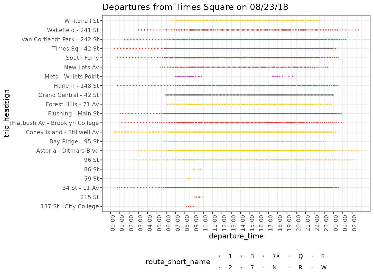
We’ll now plot all departures from Times Square depending on trip_headsign and route. We can use the route colors provided in the feed.

route_colors <- gtfs$routes %>% select(route_id, route_short_name, route_color)
route_colors$route_color[which(route_colors$route_color == "")] <- "454545"
route_colors <- setNames(paste0("#", route_colors$route_color), route_colors$route_short_name)

ggplot(departures_180823) + theme_bw() +
  geom_point(aes(y=trip_headsign, x=departure_time, color = route_short_name), size = 0.2) +
  scale_x_time(breaks = seq(0, max(as.numeric(departures$departure_time)), 3600), 
               labels = scales::time_format("%H:%M")) +
  theme(axis.text.x = element_text(angle = 90, hjust = 1)) +
  theme(legend.position = "bottom") +
  scale_color_manual(values = route_colors) +
  labs(title = "Departures from Times Square on 08/23/18")

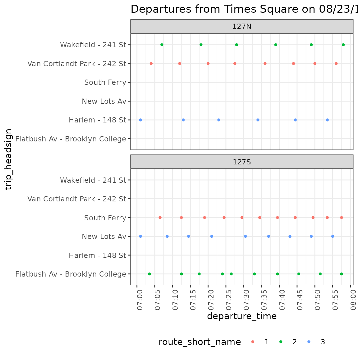
Now we plot departures for all stop_ids with the same name, so we can separate for different stop_ids. The following plot shows all departures for stop_ids 127N and 127S from 7 to 8 AM.

departures_180823_sub_7to8 <- departures_180823 %>% 
  filter(stop_id %in% c("127N", "127S")) %>% 
  filter(departure_time >= hms::hms(hours = 7) & departure_time <= hms::hms(hours = 8))

ggplot(departures_180823_sub_7to8) + 
  theme_bw() +
  geom_point(aes(y=trip_headsign, x=departure_time, color = route_short_name), size = 1) +
  scale_x_time(breaks = seq(7*3600, 9*3600, 300), labels = scales::time_format("%H:%M")) +
  scale_y_discrete(drop = FALSE) +
  theme(axis.text.x = element_text(angle = 90, hjust = 1)) +
  theme(legend.position = "bottom") +
  labs(title = "Departures from Times Square on 08/23/18") +
  facet_wrap(~stop_id, ncol = 1)

Of course this plot idea can be expanded further. You could also differentiate each route by direction (using direction_id, headsign, origin or next/previous stops). Another approach is to calculate frequencies and show different levels of service during the day, all depending on the goal of your analysis.

Flavio Poletti